Waiting Lines
What appears below is the
first model in the book (from Chapter 2, Section 1). This model is very simple; much more
elaborate models are possible. The
goal here is just to give you a feel for how SimQuick works. Explanations of the details (including
an introduction to simulation) can be found in the book.
Example: A bank
Consider the following
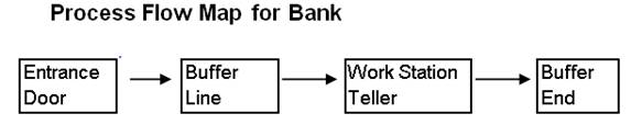
process within a small bank: Customers enter the bank, get into a single line,
are served by a teller, and finally leave the bank. Currently, this bank has one teller
working from 9 a.m. to 11 a.m. Management is concerned that the wait in
line seems to be too long. Therefore, they are considering two process
improvement ideas: adding an additional teller during these hours or installing
a new automated check-reading machine that can help the single teller serve
customers more quickly.
What should management do?
To answer this question,
management has collected and summarized some data:
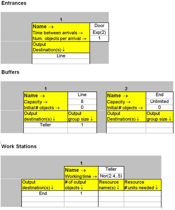
The
amount of time between arrivals of customers can be approximated by an exponential
distribution with a mean of 2 minutes.
The line in this bank can only hold 8 people and if a person arrives
when the line is full, he/she does not get in line. The service time by the teller can be
approximated by a normal distribution with a mean of 2.4 minutes and a standard
deviation of .5 minutes.
Building the model
Next we see how to build a
SimQuick model for the current process with a single teller.
SimQuick provides five
building blocks, called Elements, which can be combined in a huge number of
ways. The elements are Entrances,
Exits, Buffers, Workstations, and Decision Points.
The first step in using
SimQuick is to draw a flow map of the real-world process using these building
blocks. Here’s what the model
looks like for the bank:
The next step is to input
the model into SimQuick in Excel.
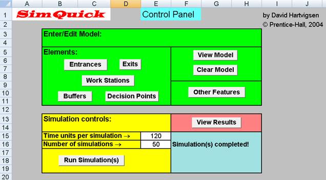
You first open the Excel file SimQuick-v2.xls. What you see is the Control Panel, which
is copied below. For each element
in the model, you click on the element’s button on the Control Panel and
fill in a table with the details about the element. You also fill in, on the Control Panel,
how many simulations you want to do and how long each simulation should last. (In this example, we are doing 50
simulations, each for 120 time units, which corresponds to two hours.) The filled-in Control Panel and tables
look like this:
Running and analyzing the model
You then click Run
Simulations on the Control Panel. It
takes SimQuick just a few seconds to simulate the 9AM to 11AM time period at
the bank 50 times. Clicking on View
Results brings up the table below.
(Here we see only the results of the first five simulations.)
|
Simulation
Results |
|
|
|
|
|
|
||
|
|
|
|
|
|
|
|
|
|
|
Element |
Element |
Statistics |
Overall |
Simulation number(s) |
||||
|
types |
names |
|
means |
1 |
2 |
3 |
4 |
5 |
|
|
|
|
|
|
|
|
|
|
|
Entrance(s) |
Door |
Objects entering process |
53.88 |
58 |
56 |
55 |
57 |
48 |
|
|
|
Objects unable to enter |
6.70 |
7 |
3 |
6 |
18 |
0 |
|
|
|
Service level |
0.90 |
0.89 |
0.95 |
0.90 |
0.76 |
1.00 |
|
|
|
|
|
|
|
|
|
|
|
Work Station(s) |
Teller |
Final status |
NA |
Working |
Working |
Working |
Working |
Not Working |
|
|
|
Final inventory (int. buff.) |
0.00 |
0 |
0 |
0 |
0 |
0 |
|
|
|
Mean inventory (int. buff.) |
0.00 |
0.00 |
0.00 |
0.00 |
0.00 |
0.00 |
|
|
|
Mean cycle time (int. buff.) |
0.00 |
0.00 |
0.00 |
0.00 |
0.00 |
0.00 |
|
|
|
Work cycles started |
48.43 |
51 |
49 |
49 |
50 |
48 |
|
|
|
Fraction time working |
0.96 |
0.98 |
1.00 |
0.97 |
0.97 |
0.96 |
|
|
|
Fraction time blocked |
0.00 |
0.00 |
0.00 |
0.00 |
0.00 |
0.00 |
|
|
|
|
|
|
|
|
|
|
|
Buffer(s) |
Line |
Objects leaving |
48.43 |
51 |
49 |
49 |
50 |
48 |
|
|
|
Final inventory |
5.45 |
7 |
7 |
6 |
7 |
0 |
|
|
|
Minimum inventory |
0.00 |
0 |
0 |
0 |
0 |
0 |
|
|
|
Maximum inventory |
7.77 |
8 |
8 |
8 |
8 |
7 |
|
|
|
Mean inventory |
4.47 |
5.03 |
4.64 |
3.05 |
6.43 |
3.42 |
|
|
|
Mean cycle time |
11.04 |
11.83 |
11.36 |
7.46 |
15.43 |
8.54 |
|
|
|
|
|
|
|
|
|
|
|
|
End |
Objects leaving |
0.00 |
0 |
0 |
0 |
0 |
0 |
|
|
|
Final inventory |
47.44 |
50 |
48 |
48 |
49 |
48 |
|
|
|
Minimum inventory |
0.00 |
0 |
0 |
0 |
0 |
0 |
|
|
|
Maximum inventory |
47.44 |
50 |
48 |
48 |
49 |
48 |
|
|
|
Mean inventory |
22.75 |
22.84 |
24.19 |
22.71 |
23.29 |
22.89 |
|
|
|
Mean cycle time |
Infinite |
Infinite |
Infinite |
Infinite |
Infinite |
Infinite |
From this table you can
see two key performance measures: Our simulated customers were waiting in line
for 11.04 minutes, on average (see the “Mean cycle time” row under
“Buffer(s), Line”), and there were 4.47 customers in line, on
average (see the “Mean inventory” row under “Buffer(s),
Line”).
From here it’s easy
to change the model for the case of two tellers and the case of a single teller
who can work faster due to some automation. We can then see the effect of these
changes on the waiting time and number of customers in line. This can help management decide what to
do.
See the book for the
details.